Exploring Public Views on Oceanic and Shoreline Ecosystem Threats Through Machine Learning

 

Catherine Ngo ¹, Orson Chi ² , Yeong Nain Chi ³ 

 

¹ Department of Agriculture, Food, and Resource Sciences University of Maryland Eastern Shore Princess Anne, MD 21853 U.S.A

² Department of Computer Science and Engineering Technology University of Maryland Eastern Shore Princess Anne, MD 21853    U.S.A

³ Department of Agriculture, Food, and Resource Sciences University of Maryland Eastern Shore Princess Anne, MD 21853 U.S.A

 

1. INTRODUCTION

Oceanic and shoreline ecosystems (e.g., coral reefs, salt marshes, rocky shores, and estuaries) are essential in preserving ecological stability and promoting biodiversity. These ecosystems act as nurseries for many marine species, provide habitat for a wide range of organisms, and contribute to the livelihoods of millions of people worldwide. They also offer critical services such as carbon sequestration, which helps mitigate climate change, and coastal protection, which reduces the impact of storms and erosion on coastal communities.

Despite their significance, marine and coastal ecosystems face numerous threats from human activities and environmental changes. Some of the most notable threats include overfishing, plastic pollution, climate change, shipping, and coastal development. However, they face escalating threats from human activities, including overfishing FAO, 2021, pollution Barnes et al. (2020), habitat destruction Worm et al. (2021), and climate change Claudet et al. (2018)  (IPCC). (2022). These challenges are compounded by anthropogenic factors like industrial development, urbanization, and intensified exploitation of marine resources Halpern et al. (2019); Levin & Möllmann (2020).

Public perceptions of environmental threats play a crucial role in shaping conservation efforts and policy decisions. Understanding how the public perceives the severity of various threats to marine and coastal ecosystems can help policymakers and conservationists design more effective and targeted strategies. Public awareness and concern for environmental issues can drive political will and funding for conservation initiatives, making it essential to align public perceptions with scientific understanding and conservation priorities.

Public perceptions of threats to marine and coastal ecosystems vary significantly based on factors such as geographic location, socioeconomic background, education level, and proximity to marine environments. For example, communities reliant on marine resources for their livelihoods may demonstrate heightened awareness of overfishing and habitat degradation. Conversely, urban populations might perceive marine threats through the lens of recreational or aesthetic value, often neglecting deeper ecological implications.

While previous studies Lotze et al. (2018); Thompson & Williams (2019) have provided valuable insights, a comprehensive understanding of how diverse populations perceive threats to oceanic and shoreline ecosystems remains limited. The study’s primary objective was to classify respondents based on their perceptions using principal component analysis (PCA)-based k-means clustering.

PCA is a statistical approach that converts the data into a set of orthogonal components, which helps in minimizing the scope of the data while maintaining most of its variability. K-means clustering is a method used to partition the data into distinct groups or clusters based on the similarities in their responses. By combining these two techniques, the study was able to identify three distinct clusters of participants, each reflecting different perspectives on the severity of the dangers to oceanic and shoreline ecosystems.

Understanding public perceptions of the significant dangers to oceanic and shoreline ecosystems is critical for fostering informed decision-making and mobilizing collective action. This study could contribute to the expanding body of literature by offering a data-driven exploration of public awareness and attitudes, underscoring the importance of aligning conservation strategies with societal values and priorities.

 

2. DATA

This study leverages data from the publicly accessible dataset titled "Marine and Coastal Ecosystems and Climate Change: Dataset from a Public Awareness Survey" (https://data.mendeley.com/datasets/t82xdzpdh8/2) to explore public perceptions of major threats to oceanic and shoreline ecosystems. The survey was derived from a self-conducted online questionnaire exploring public views of climate change, the perceived value and threats to oceanic and shoreline ecosystems, climate change response opinions, and socio-demographic characteristics of respondents Fonseca et al. (2022) Fonseca et al. (2023). Conducted in English, French, Spanish, and Italian, the survey included a participant information form in these languages.

The survey gathered responses from a diverse group of participants who assessed the severity of 13 significant threats, including fishing, plastic pollution, climate change, shipping, and coastal development. These threats were evaluated using a psychometric rating scale of 1 (very low) to 5 (very high), with an additional option for "I don't know." The study aimed to evaluate the psychometric properties of the threat scale related to marine and coastal ecosystems, analyzing data from 709 respondents who provided complete responses to all 13 threat-related statements Table 1

Table 1

Table 1 Descriptive Statistics of Marine and Costal Ecosystems Threat Scale
Please rate the following threats to marine and coastal ecosystems in your country as to how serious you feel the threat is:	Mean	S.D.
Fishing / harvesting of marine and / or coastal life	4.11	0.88
Extraction of non-living resources (e.g., sand, aggregates, minerals)	3.76	1.19
Plastic pollution	4.43	0.80
Shipping	3.77	0.98
Climate change	4.4	0.76
Coastal development	3.98	0.96
Tourism / recreation	3.61	1.00
Aquaculture	3.47	1.26
Land runoff	4.15	1.17
Marine noise	3.78	1.32
Invasive species	3.95	1.07
Chemical pollution	4.17	0.95
Other infrastructure (e.g., renewable energy, communications)	3.42	1.30
(Very Low = 1, Low = 2, Medium = 3, High = 4, Very High = 5, I don’t know = 6)

 

3. METHODOLOGY

This research adopts a systematic methodology that synergizes PCA with k-means clustering to elucidate patterns within the dataset. This approach establishes a robust framework for dimensionality reduction, optimal cluster determination, and the interpretation of significant groupings.

 

3.1.  DATA PROCESSING

The dataset is meticulously pre-processed to ensure analytical suitability. Initially, missing data is addressed through statistical imputation or exclusion to maintain dataset integrity. Features are standardized to a mean of 0 and a standard deviation of 1, a critical step for both PCA and k-means clustering. This standardization mitigates biases from varying feature scales, allowing PCA to effectively capture variance and ensure accurate distance calculations in k-means clustering. A thorough feature selection process is also conducted to eliminate redundancies and retain variables most pertinent to the study's objectives.

 

 

 

 

3.2. DIMENSIONALITY REDUCTION WITH PCA

Principal Component Analysis (PCA) is applied to minimize the scope of the dataset while maintaining as much variance as possible. This process begins with the computation of PCA components, which involves transforming the original variables into a new set of orthogonal components. Each component captures a portion of the total variance present in the dataset. The explained variance ratio is then analyzed to determine the optimal number of components to retain, assuring that the selected components account for a substantial proportion of the total variance. This balance between dimensionality reduction and information retention is crucial for maintaining the integrity of the data.

Once the appropriate components are selected, the dataset is projected into this reduced-dimensional PCA space. This transformation facilitates the subsequent clustering process by simplifying the dataset, reducing computational complexity, and minimizing noise. By focusing on the most informative components, PCA enhances the efficiency and accuracy of clustering algorithms, such as k-means, recognizing meaningful patterns and groupings within the data.

 

3.3. K-MEANS CLUSTERING APPLICATION

Following the transformation into the PCA space, the k-means clustering algorithm is applied to the dataset. This process involves iterating over a range of potential cluster counts and executing the k-means algorithm for each specified number of clusters. The k-means algorithm works by organizing data points into clusters in such a way that the sum of squared errors (SSE) within each cluster is minimized. This is achieved by assigning each data point to the nearest cluster centroid, followed by recalculating the centroids based on the mean of the assigned points.

During this iterative operation, multiple clustering outcomes are generated, each corresponding to a different number of clusters. These outcomes include cluster labels, which indicate the cluster membership of each data point; centroids, which represent the center of each cluster; and inertia values, which measure the total SSE within the clusters. These initial clustering results are crucial for subsequent analyses, as they provide a foundation for evaluating the appropriate amount of distinct groups and the overall quality pertaining to the clustering solution.

The evaluation of these clustering outcomes involves assessing various metrics and criteria to determine the most appropriate number of clusters. Techniques such as the elbow method, silhouette analysis, and gap statistics may be employed to identify the point at which adding more clusters does not significantly improve the clustering quality. By thoroughly analyzing these metrics, the study ensures that the final clustering solution is both robust and meaningful, providing crucial information about the data’s underlying framework.

 

3.4.  DETERMINING THE OPTIMAL NUMBER OF CLUSTERS

The determination of the optimal cluster count (k) is a critical step in the clustering process, and it is achieved through the application of several robust evaluation techniques:

1)    The Elbow Method: This technique incorporates marking the sum of squared error (SSE) values against the number of clusters. The "elbow point" on the plot is identified as the point where the addition of more clusters results in a diminishing improvement in SSE. This point indicates the optimal number of clusters, balancing model complexity and fit.

2)    The Average Silhouette Score: This method analyzes the clustering quality by measuring both intra-cluster cohesion and inter-cluster separation. The silhouette score ranges from -1 to 1, with higher values indicating better-defined clusters. The optimal number of clusters is selected based on the k value that maximizes the average silhouette score, ensuring well-separated and cohesive clusters.

3)    The Gap Statistic: This technique compares the clustering results to a null reference distribution of the data. By calculating the gap statistic for a range of figures for k, this method identifies the cluster count that maximizes the gap statistic, indicating the most appropriate clustering solution relative to the null model.

4)    The NbClust () Function: This comprehensive function aggregates results from multiple clustering indices to provide a well-rounded recommendation for the optimal number of clusters. By considering various criteria and indices, the NbClust() function ensures a thorough and reliable determination of the best k value.

These complementary methods collectively ensure a robust and consistent approach to determining the optimal cluster count. By leveraging multiple evaluation techniques, the study enhances the reliability and validity of the clustering results, providing a solid foundation for subsequent analyses and interpretations.

 

3.5. VISUALIZATION AND REPORTING

To enhance the interpretability of the clustering results, clusters are visualized in the reduced PCA space using scatterplots. These visualizations provide a clear and intuitive representation of the data, allowing for the identification of distinct clusters and the relationships between them. Additionally, a biplot is employed to illustrate how the original features contribute to the principal components. This biplot aids in understanding how the original variables influence the clustering results, offering insights into the underlying structure of the data.

The findings are further summarized by reporting the optimal number of clusters, determined through rigorous evaluation methods. This comprehensive approach ensures that the chosen clustering solution is both meaningful and robust. By combining visualizations with detailed analysis, the study provides a thorough and systematic exploration of the data, facilitating a deeper understanding of the clustering outcomes.

This methodology not only enhances the clarity and interpretability of the results but also maintains methodological integrity. By employing advanced analytical techniques and robust evaluation methods, the study yields valuable insights into the dataset while ensuring the reliability and validity of the findings. This systematic approach to data exploration and cluster analysis underscores the importance of integrating visualization tools with statistical methods to derive actionable insights from complex datasets.  

 

 

 

 

4. RESULTS

4.1.  PRINCIPAL COMPONENT ANALYSIS (PCA)

Eigenvalues serve as an essential function in PCA by quantifying variation amounts captured by each principal component, thereby serving as a measure of their significance. Typically, the largest eigenvalue corresponds to the first principal component, which aligns with the direction of maximum variation in the dataset. Subsequent principal components, each associated with progressively smaller eigenvalues, capture decreasing amounts of variation. This hierarchical capture of variance allows for a structured reduction in dimensionality while retaining the most critical information.

In this study, eigenvalues were meticulously analyzed to identify the most suitable number of principal components to retain. This analysis involved examining the eigenvalues and their corresponding explained variance ratios to identify the components that collectively account for a substantial proportion of the dataset's total variance. By retaining components with significant eigenvalues, the study ensures that the reduced-dimensional representation of the data maintains its integrity and informational value.

Table 2 presents a detailed summary of the eigenvalues and the proportion of variance explained by each principal component. The dataset’s total variance is represented by the sum of all eigenvalues, which in this case totals 10. This comprehensive analysis of eigenvalues not only facilitates the dimensionality reduction process but also enhances the interpretability and robustness of the subsequent clustering analysis.

Table 2

Table 2  Eigenvalues, Variance %, and Cumulative Variance %
	Eigenvalue	Variance %	Cumulative Variance %
Dim. 1	4.0999074	31.537749	31.53775
Dim. 2	1.2259311	9.430239	40.96799
Dim. 3	1.1247139	8.651646	49.61963
Dim. 4	0.8881689	6.832069	56.4517
Dim. 5	0.8274571	6.365055	62.81676
Dim. 6	0.7930924	6.100711	68.91747
Dim. 7	0.7197588	5.536606	74.45407
Dim. 8	0.6715601	5.165847	79.61992
Dim. 9	0.6230192	4.792455	84.41238
Dim. 10	0.5870628	4.515868	88.92825
Dim. 11	0.5206575	4.005058	92.9333
Dim. 12	0.4944198	3.803229	96.73653
Dim. 13	0.4242509	3.263468	100.00000

 

The second column of the table presents the proportion of variation explained by each eigenvalue. For instance, dividing an eigenvalue of 4.100 by the total variance of 10 yields 0.4100, indicating that approximately 41.00% of the variation is explained by the first principal component. The cumulative percentage of variation explained is calculated by successively adding these proportions to obtain a running total. For example, adding 31.53775% to 9.430239% results in 40.96799%. Consequently, the first two eigenvalues together account for approximately 40.97% of the total variation.

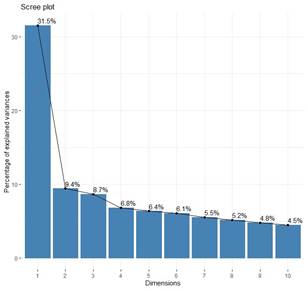
Determining the appropriate number of principal components to retain is a subjective process that varies by field of study and the specific dataset in question. In practice, the first few principal components are often examined to identify meaningful patterns in the data. A common approach to this decision is the use of a scree plot, which displays the eigenvalues in descending order. The optimal number of components is identified at the point where the eigenvalues level off, indicating that the remaining components account for relatively small and comparable variances.

In this study, the first two principal components explained approximately 41% of the variation. To facilitate the selection of principal components for further analysis, a scree plot was generated to visually assess the eigenvalues and their corresponding variances Figure 1. This visual representation aids in identifying the point at which additional components contribute minimally to the overall variance, thereby guiding the decision on the number of components to retain.

The correlation between a variable and a principal component is indicative of the variable's coordinate on that component, reflecting its contribution to the principal component's variance. Unlike observation plots, where individual data points are depicted by their projections onto the principal components, variables are illustrated through their correlations with these components. This type of visualization, known as a variable correlation plot Figure 2, elucidates the interrelationships among variables and their contributions to the principal components.

The variable correlation plot can be interpreted as follows:

·        Variables with positive correlations are clustered together, indicating that they contribute similarly to the principal component and tend to vary in the same direction.

·        Variables with negative correlations are situated on opposite sides of the plot origin, typically in opposing quadrants. This positioning signifies that these variables contribute in opposite directions to the principal component.

·        The distance from the origin signifies the quality of the variable's representation on the factor map. Variables positioned further from the origin are more accurately represented by the principal component, whereas those nearer to the origin exhibit weaker correlations and contribute less to the component's variance.

Furthermore, a biplot Figure 3 integrates variable correlations with observations, providing a comprehensive visual representation of the relationships between variables and individual data points. This dual representation enhances the understanding of principal components by illustrating how variables contribute to the patterns observed within the data. The biplot effectively combines the insights from both the variable correlation plot and the observation plot, offering a holistic view of the data structure and the underlying relationships.

Figure 1

Figure 1 PCA Screen Plot

 

Figure 2

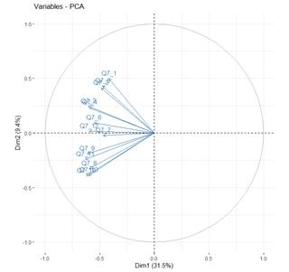
Figure 2 Variables – PCA Plot

 

Figure 3

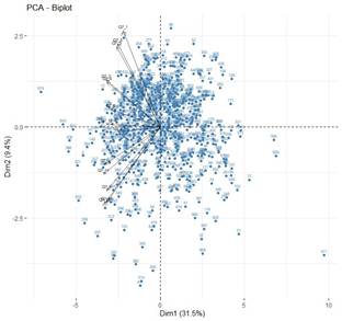
Figure 3 PCA – Biplot Plot

 

 

4.2.  K-MEANS CLUSTERING

4.2.1.  ELBOW METHOD

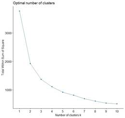
The elbow method is a widely utilized technique to determine the appropriate amount of clusters in a dataset by assessing the total within-cluster sum of squares (WSS), also known as total intra-cluster variation, relative to the number of clusters. WSS quantifies the compactness of the clustering, with lower values indicating more cohesive clusters. The process for identifying the optimal cluster count using the elbow method involves several steps:

1)    Implementing a Clustering Algorithm: Apply a clustering algorithm, such as k-means, for a range of different k values (the number of clusters).

2)    Calculating Total WSS: For each k value, calculate the total WSS, which measures the sum of squared distances between each data point and its corresponding cluster centroid.

3)    Plotting WSS Values: Plot the WSS values against the number of clusters (k) to create an elbow plot.

4)    Identifying the "Elbow" Point: Locate the "elbow" or "knee" on the plot, which is the point where the rate of decrease in WSS significantly diminishes. This point indicates the optimal number of clusters, as adding more clusters beyond this point results in minimal improvement in clustering compactness.

In this analysis, the elbow method identified an optimal solution of 2 clusters Figure 4. However, it is important to note that the elbow method may produce ambiguous outcomes if the bend in the plot is indistinct or gradual. In such cases, additional validation techniques can be employed to ensure the robustness of the clustering solution.

One alternative validation method is the average silhouette score, which analyzes the caliber of the clusters based on both intra-cluster cohesion and inter-cluster separation. The silhouette score ranges from -1 to 1, with higher values indicating better-defined clusters. By calculating the average silhouette score for different k values, this method provides a complementary assessment of cluster quality further validating the optimal number of clusters identified by the elbow method.

By employing these complementary techniques, the study ensures a robust and consistent approach to determining the optimal cluster count, thereby enhancing the reliability and validity of the clustering results.

Figure 4

Figure 4 Optimal Number of Clusters Using Elbow Method

 

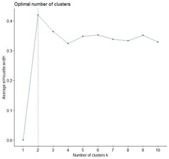
4.2.2.  AVERAGE SILHOUETTE SCORE METHOD

The average silhouette score method provides a robust technique for assessing clustering quality by determining the average silhouette score for various values of k, as described by Kaufman & Rousseeuw (2005). This method identifies the optimal cluster count as the k value that maximizes the silhouette score. This approach parallels the elbow method, involving these steps:

1)    Implement a Clustering Algorithm: Apply a clustering algorithm, such as k-means, for a series of different k values (the number of clusters).

2)    Calculate the Average Silhouette Score: For each k value, calculate the average silhouette score, which measures the clustering quality by evaluating intra-cluster cohesion and inter-cluster separation.

3)    Graph the Average Silhouette Score: Plot the average silhouette score against the number of clusters to create a silhouette plot.

4)    Determine the Optimal k Value: Identify the k value where the silhouette score peaks, indicating the optimal cluster count.

The silhouette score evaluates the separation of points within a cluster from those in adjacent clusters, with higher scores signifying more distinct and cohesive clusters. A silhouette score close to 1 demonstrates that the data points are well-clustered, while a score close to -1 implies that the data points could have been placed in the incorrect group. The silhouette plot offers a visual representation of this metric, enhancing the understanding of clustering quality and contributing to identifying the most suitable number of clusters.

In this analysis, the average silhouette score method determined that the optimal solution is two clusters Figure 5. This method provides a quantitative and visually intuitive complement to the elbow method for assessing the appropriate amount of clusters. By leveraging both the elbow method and the average silhouette score method, this study ensures a robust and comprehensive approach to cluster validation, thereby enhancing the reliability and interpretability of the clustering results.

Figure 5

 

Figure 5 Optimal Number of Clusters Using Average Silhouette Score Method

 

 

 

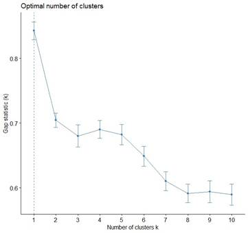
4.2.3.   GAP STATISTIC METHOD

The gap statistic method thoroughly evaluates the total within-cluster variation across different cluster counts (k) by assessing them relative to the expected values obtained from a null reference distribution, as outlined by Tibshirani et al. (2001). This method identifies the optimal cluster count as the k value that maximizes the gap statistic, indicating a significant deviation from a random uniform distribution of data points. This algorithm involves several key steps:

1)    Clustering the Observed Data: The observed data is clustered using varying values of k.

2)    Generating Reference Datasets: B reference datasets are generated, each with a random uniform distribution of data points.

3)    Calculating the Gap Statistic: For each k, the gap statistic is calculated as the difference between the observed within-cluster variation and the expected variation from the reference datasets.

An optimal k is selected as the smallest value where the gap statistic is within one standard deviation of the maximum gap value. This approach ensures that the chosen number of clusters represents a significant improvement over random clustering, providing a statistically robust framework for determining the optimal number of clusters.

Unlike the elbow and average silhouette score methods, which lack formal statistical grounding, the gap statistic method offers a more rigorous and statistically sound approach to cluster validation. In this study, the analysis indicated an optimal solution of one cluster, underscoring the method's statistical robustness and its ability to provide reliable insights into the data's underlying structure.

Figure 6

Figure 6 Optimal Number of Clusters Using Gap Statistic Method

 

4.2.4.   NBCLUST () METHOD

The NbClust() function, integral to the NbClust package in R Charrad et al. (2014), serves as an advanced tool for calculating the optimal number of clusters within clustering algorithms. This function meticulously evaluates 30 distinct indices, identifying the most appropriate number of clusters, subsequently recommending the most suitable clustering scheme based on the derived outcomes. By leveraging NbClust(), users can explore various permutations of cluster numbers, distance metrics, and clustering methodologies, thereby enhancing the robustness of their analysis.

One of the notable advantages of NbClust() is its ability to compute all indices concurrently, significantly streamlining the process of determining the optimal number of clusters through a single function invocation. This capability not only enhances the efficiency of the clustering analysis but also ensures consistency and reliability in the results. The comprehensive assessment provided by NbClust() is pivotal in achieving meaningful and dependable clustering outcomes.

In this investigation, the majority rule was employed across the computed indices to determine the optimal number of clusters. This analysis identified three clusters as the most suitable solution Figure 7. This methodical approach, facilitated by NbClust(), underscores the importance of using advanced analytical tools to derive actionable insights from complex datasets.

Figure 7

Figure 7 Optimal Number of Clusters Using NbClust () Function

 

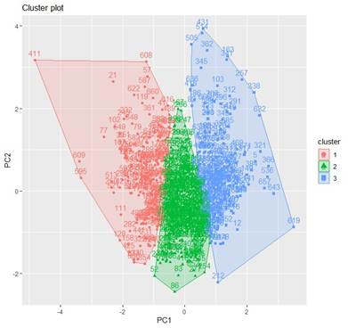
5.   FINDINGS

In this study, a PCA-based k-means clustering approach was utilized to determine the optimal solution with a specified number of clusters. Consequently, a solution comprising of three clusters was chosen, as illustrated in Table 3, Figure 8, and Figure 9.

Table 3

Table 3 Cluster Means Using K-Means Clustering
Cluster	PC1	PC2	Total
Cluster 1	-2.64602311	0.3811266	169
Cluster 2	-0.08132256	-0.4932817	330
Cluster 3	2.25721119	0.4684407	210

 

Figure 8

Figure 8 Cluster Plot of the Three Identified Clusters

 

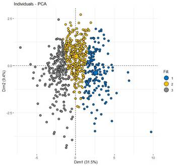
Figure 9

Figure 9 Individuals - PCA Plot of the Three Identified Clusters

 

The analysis revealed three distinct clusters of participants. The first cluster consisted of respondents who perceived the threats as less severe, possibly indicating a lower level of awareness of concern for these issues. The second cluster included participants who rated most threats as moderately severe, suggesting a balanced view of the environmental risks. The third cluster comprised individuals who perceived all threats as highly severe, indicating a heightened awareness and concern for marine and coastal conservation. This clustering provided valuable insights into the diverse ways different population segments perceive and prioritize environmental risks.

Upon identifying the three clusters, a series of statistical tests were conducted to explore the relationships between these clusters and various demographic factors, including gender, age group, educational level, and the severity of 13 significant threats. To assess the significant differences between female and male respondents across the three clusters, the Chi-square test was applied. The results indicated significant gender differences among the clusters (χ² = 33.680, df = 6, p < 0.001) at a significance level of 0.01. Conversely, the results showed no significant differences in age group (χ² = 9.729, df = 10, p = 0.465) and educational level (χ² = 14.903, df = 10, p = 0.136) among the clusters at a significance level of 0.05. Additionally, significant differences were observed in the severity of all 13 significant threats across the three clusters, as determined by the Chi-square test at a significance level of 0.01 Table 4

Table 4

Table 4 Chi-Square Test of Marine and Costal Ecosystems Threat Scale Among the Clusters
	Chi-Square	df	p
Fishing / harvesting of marine and / or coastal life	147.427	10	< 0.001
Extraction of non-living resources (e.g., sand, aggregates, minerals)	241.86	10	< 0.001
Plastic pollution	164.936	10	< 0.001
Shipping	218.946	10	< 0.001
Climate change	150.42	10	< 0.001
Coastal development	181.648	10	< 0.001
Tourism / recreation	111.907	10	< 0.001
Aquaculture	286.119	10	< 0.001
Land runoff	275.451	10	< 0.001
Marine noise	321.91	10	< 0.001
Invasive species	280.44	10	< 0.001
Chemical pollution	236.368	10	< 0.001
Other infrastructure (e.g., renewable energy, communications)	279.582	10	< 0.001
(Very Low = 1, Low = 2, Medium = 3, High = 4, Very High = 5, I don’t know = 6)

 

6. DISCUSSION AND CONCLUSION

The methodology employed in this study effectively simplified the complexity of the dataset and revealed meaningful patterns that traditional methods might have overlooked. By utilizing multiple cluster evaluation techniques, the study ensured the reliability and robustness of the results, providing a solid foundation for data interpretation. This research highlights the utility of advanced analytical tactics, such as principal component analysis (PCA) and k-means clustering, in environmental studies. These methods reduce dimensionality and identify natural groupings within the data, offering a structured approach to understanding complex datasets. The robustness of the clustering results, validated through various evaluation methods, reinforces the credibility of the results; and underscores the capability of integrating machine learning techniques with environmental research to derive actionable insights.

The study's findings provide significant insights into public perceptions of threats to marine and coastal ecosystems, carrying crucial implications for environmental policy and management. The application of principal component analysis (PCA) and k-means clustering helped identify distinct groups of respondents with shared perceptions, thereby enhancing the understanding of the diversity in public attitudes. This approach highlighted varying levels of awareness and concern regarding threats such as climate change, pollution, and overfishing, underscoring the necessity for tailored conservation strategies for different audience segments. These findings not only enrich the literature on environmental perceptions but also offer actionable recommendations for policymakers and conservation practitioners.

By mapping these perceptions, the study offers critical guidance for policymakers and conservationists. The findings emphasize the need for tailored, data-driven strategies in environmental conservation and marine protection. For instance, public awareness campaigns can be designed to target specific clusters, addressing their unique concerns and knowledge gaps. Additionally, the insights from this study can inform the development of policies that align public concern with effective climate change mitigation efforts and targeted interventions to safeguard marine ecosystems.

The study highlights the importance of engaging the public in conservation efforts. By understanding how different segments of the population perceive environmental threats, policymakers can foster greater public support for conservation initiatives. This engagement is essential for the successful implementation of policies aimed at protecting marine and coastal ecosystems. The study also underscores the need for continuous monitoring of public perceptions, as these can change over time in response to newly added information and environmental events.

In conclusion, this research provides a comprehensive analysis of public perceptions of threats to oceanic and shoreline ecosystems. The use of PCA-based k-means clustering has revealed distinct patterns in how different population segments view these threats, offering valuable insights for policymakers and conservationists. By leveraging these insights, it is possible to develop more effective and targeted strategies for environmental conservation, contributing to the protection and sustainability of marine and coastal ecosystems.

Future insights from this study can guide targeted awareness campaigns addressing specific concerns and knowledge gaps within different population segments. The demonstrated methodological framework can be applied to other environmental issues, improving public perception and understanding in various contexts. By aligning public attitudes with conservation efforts, this research supports sustainable management and protection of marine and coastal ecosystems, critical priorities amid escalating environmental threats.

 

7. FUNDINGS

This project is funded by the USDA National Institute of Food and Agriculture in collaboration with the 1890 Center of Excellence for Emerging IoT Technologies for Smart Agriculture.

 

CONFLICT OF INTERESTS

None. 

 

ACKNOWLEDGMENTS

None.

 

REFERENCES

Barnes, S. J., Wallis, C., & Andrews, L. (2020). Global Marine Plastic Pollution: A Comprehensive Meta-Analysis of Microplastic Contamination. Marine Pollution Bulletin, 153, 110994. https://doi.org/10.1016/j.marpolbul.2020.110994

Charrad, M., Ghazzali, N., Boiteau, V., & Niknafs, A. (2014). NbClust: An R Package for Determining the Relevant Number of Clusters in a Data Set. Journal of Statistical Software, 61(6), 1-36. https://doi.org/10.18637/jss.v061.i06

Claudet, J., Bopp, L., Cheung, W. W., et al. (2018). Interconnections between Global Ocean Ecosystems Under Anthropogenic Climate Change. Nature Climate Change, 8(6), 484-492.

Fonseca, C., Wood, L., Andriamahefazafy, M., Casal, G., Chaigneau, T., Cornet, C. C., Degia, A., Pierre, F., Ferraro, G., Furlan, E., Hawkins, J., de Juan, S., Krause, T., McCarthy, T., Pérez, G., Roberts, C., Tregarot, E., & O'Leary, B. C. (2022). Marine and Coastal Ecosystems and Climate Change: Dataset from a Public Awareness survey. Mendeley Data, V2. https://doi.org/10.17632/t82xdzpdh8.2

Fonseca, C., Wood, L., Andriamahefazafy, M., Casal, G., Chaigneau, T., Cornet, C. C., Degia, A., Pierre, F., Ferraro, G., Furlan, E., Hawkins, J., de Juan, S., Krause, T., McCarthy, T., Pérez, G., Roberts, C., Tregarot, E., & O'Leary, B. C. (2023). Survey Data of Public Awareness on Climate Change and the Value of Marine and Coastal Ecosystems. Data in Brief, 47, 108924, 1-9. https://doi.org/10.1016/j.dib.2023.108924

Food and Agriculture Organization (FAO). (2021). The State of World Fisheries and Aquaculture 2020. Rome, FAO.

Halpern, B. S., Frazier, M., Potapenko, J., et al. (2019). Spatial and Temporal Changes in Cumulative Human Impacts on the World's Ocean. Nature Communications, 10(1), 1-11.

Intergovernmental Panel on Climate Change (IPCC). (2022). Climate Change 2022: Impacts, Adaptation and vulnerability. Cambridge University Press. https://doi.org/10.1017/9781009325844

Kaufman, L., & Rousseeuw, P. J. (2005). Finding Groups in Data: An Introduction to Cluster Analysis. Hoboken, NJ: John Wiley & Sons.

Levin, P. S., & Möllmann, C. (2020). Marine Ecosystem Regime Shifts: Challenges and Opportunities for Ecosystem-Based Management. Philosophical Transactions of the Royal Society B, 375(1814), 20190349.  

Lotze, H. K., Guest, H., O'Leary, J., Tuda, A., & Wallace, D. (2018). Public Perceptions of Marine Threats and Protection from Around the world. Ocean & Coastal Management, 152, 14-22. https://doi.org/10.1016/j.ocecoaman.2017.11.004

Thompson, R. C., & Williams, A. T. (2019). Public Perceptions and Environmental Awareness of Marine Ecosystem Threats. Ocean & Coastal Management, 172, 86-97.

Tibshirani, R., Walther, G., & Hastie, T. (2001). Estimating the Number of Clusters in a Data Set Via the Gap Statistic. Journal of the Royal Statistical Society Series B: Statistical Methodology, 63(2), 411-423. https://doi.org/10.1111/1467-9868.00293

Worm, B., Barbier, E. B., Beaumont, N., et al. (2021). Impacts of Biodiversity Loss on Ocean Ecosystem Services. Science, 314(5800), 787-790. https://doi.org/10.1126/science.1132294