9An ARIMA-NARNN Hybrid Time Series Analysis of Daily Bitcoin Price During and After the COVID-19 Pandemic Outbreak

 

Catherine Ngo ¹, Orson Chi ², Yeong Nain Chi ¹

 

¹ Department of Agriculture, Food, and Resource Sciences, University of Maryland Eastern Shore, Princess Anne, MD 21853, U.S.A

² Department of Computer Science and Engineering Technology, University of Maryland Eastern Shore, Princess Anne, MD 21853, U.S.A

 

1. INTRODUCTION

Bitcoin (BTC) is a decentralized digital currency that allows for peer-to-peer transactions without the need for a central authority or middleman. Created in 2008 by an individual or group of individuals using the alias Satoshi Nakamoto, Bitcoin was designed to build a decentralized, trust-less transaction system that eliminates the need for intermediaries such as banks Laurent (2025).

Since its creation in 2009, Bitcoin has exhibited significant price volatility, experiencing dramatic fluctuations. Despite this volatility, the growth rate of Bitcoin has been remarkable. Some analysts argue that the adoption rate of Bitcoin is outpacing that of the Internet in the 1990s, with projections suggesting that Bitcoin could reach one billion users in half the time it took the Internet to achieve the same milestone Hozjan (2025). This rapid growth stems from the financial and corporate sectors’ increasing recognition and adoption.

This acceptance is evident in the increasing number of institutional investments and endorsements from major corporations. PricewaterhouseCoopers (PwC), one of the world’s largest accounting firms, accepted their first Bitcoin payment in 2017 Russolillo (2025). For example, Tesla has invested $1.5 billion in Bitcoin in 2021 and will also start accepting it as a payment mode Ponciano (2025). Some speculations compared to the Internet; Bitcoin will take half the time to cross the one-billion-user mark Portfolio Insider (2025).

Due to the growing impact of Bitcoin in the financial and corporate world, researchers have developed complex mathematical, advanced analytics, and machine learning models to forecast its value Atsalakis et al. (2019). Traditional methods, such as the ARIMA model, have been employed to predict Bitcoin prices. For example, Ayaz et al. (2020) used the ARIMA model for their predictions, while Yenidogan et al. (2018) combined the PROPHET and ARIMA models to enhance the accuracy of their forecasts.

Researchers have recently shifted toward newer methods to improve the accuracy of Bitcoin price forecasts Luc Minh et al. (2024). Hybrid models, which combine multiple forecasting techniques, have gained popularity. These models leverage the strengths of individual methods to provide robust predictions Hajirahimi and Khashei (2023). For instance, Fathi (2025) applied a hybrid model combining ARIMA and LSTM networks to forecast the values of Wolf’s Sunspot data and the USD/GBP exchange rate.

Similarly, Hao and Gao (2020) concluded that a hybrid model consisting of three LSTM recurrent neural networks outperformed traditional forecasting models in predicting stock market trends. This finding highlights the potential of hybrid models in capturing complex patterns in financial time series data. Dowe et al. (2025) used the ARFIMA-ANN hybrid model to forecast financial, environmental, climate, and energy data in practice.

Zhang (2003) explored the use of a hybrid model combining traditional ARIMA and NARNN to predict the values of Wolf’s sunspot data, Canadian lynx data, and the USD/GBP exchange rate. This study recommends that combining ARIMA and NARNN models could effectively forecast complex datasets with both linear and nonlinear components. This hybrid approach leverages the unique strengths of ARIMA and NARNN in modeling linear components and capturing nonlinear patterns, respectively.

The field of time series research on Bitcoin is rapidly evolving, with hybrid models, machine learning, and deep learning approaches showing significant promise Boozary et al. (2025). By combining traditional statistical methods with advanced computational techniques, more accurate and robust models for predicting Bitcoin prices can be developed. These advancements not only enhance our understanding of the market dynamics of Bitcoin but also provide valuable tools for investors and financial analysts.

 

2. MATERIALS

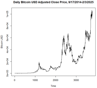
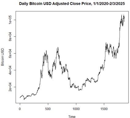
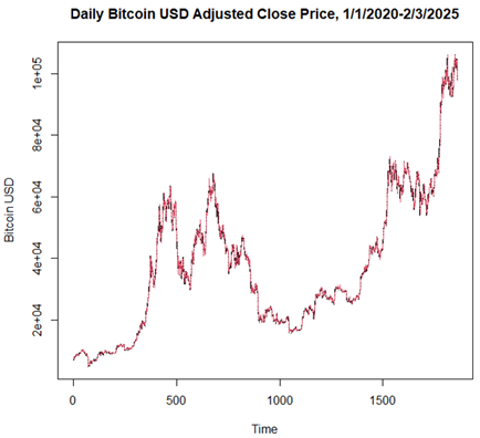
Daily Bitcoin (BTC) prices in USD are available and publicly accessible online. In this study, historical data for daily BTC-adjusted close price (USD) were taken from the official website of Yahoo! Finance (https://finance.yahoo.com/). The data in this study range from September 17, 2014, to February 3, 2025. Since the outbreak of COVID-19, during and after, the daily Bitcoin price trend showed a dramatic steep rise, and prices have been fluctuating much more than in the previous period. Figure 1 shows a graphical representation of the daily trend of Bitcoin’s adjusted close prices from September 17, 2014, to February 3, 2025. Figure 2 shows a graphical representation of the daily trend of Bitcoin’s adjusted close prices during and after the COVID-19 pandemic (January 1, 2020 - February 3, 2025).

Figure 1

Figure 1 Daily Bitcoin Adjusted Close Price (September 17, 2014 - February 3, 2025)

 

Figure 2

Figure 2 Daily Bitcoin-Adjusted Close Price During and After the COVID-19 Pandemic Outbreak (January 1, 2020 - February 3, 2025)

 

3. METHODS

3.1. AUTO-REGRESSIVE INTEGRATED MOVING AVERAGE MODEL

The ARIMA model is a popular statistical method used for time-series forecasting. It captures the linear aspects of the data using three main components:

1)    Auto-regressive (AR): This part uses the dependency between an observation and some lagged observations (previous values).

2)    Integrated (I): This involves differencing the data to make it stationary (i.e., removing trends and seasonality).

3)    Moving Average (MA): This part uses the dependency between an observation and a residual error from a MA model applied to lagged observations.

The ARIMA(p,d,q) model can be mathematically represented as follows:

 

 

where p = number of lag observations or the order for the autoregression, d = order of differencing made to make the data stationary for the non-stationary series, and q = order of the moving average, Φ = the coefficient of the auto-regressive process, θ = the coefficient of the moving average, and e is the residual error.

 

3.2. NONLINEAR AUTOREGRESSIVE NEURAL NETWORK MODEL

The NARNN model is a type of ANN designed to handle nonlinear relationships in time series data. It uses the past time series values to predict future values. The AR process of order p is given by

 

 

Since the NARNN models are natural approximator and have high generalization ability, the NARNN model can be written as follows:

 

 

where Φ is the function determined by the neural network as it processes the data, w represents the weights, and e represents the error term.

The NARNN model has two major components. The first is the neurons in the hidden layer, which are the processing units in the neural network that help capture complex patterns in the data. Time Delays represent the lagged inputs used to predict future values. For example, two-time delays mean the model uses the past two observations to make predictions.

 

 

 

 

3.3. ARIMA-NARNN HYBRID MODEL

The basic limitations of the ARIMA and NARNN models are that they are effective in modeling linear and nonlinear time series, respectively. Therefore, modeling and forecasting time series data using ARIMA or NARNN alone generates higher errors and reduces the overall accuracy Denton (1995). The hybrid model combines the strengths of two approaches: the ARIMA and NARNN models. It leverages both linear and nonlinear modeling capabilities as follows:

·        ARIMA Component: First, the ARIMA model is applied to the time series data to capture and model the linear patterns.

·        NARNN Component: The residuals (errors) from the ARIMA model are then fed into the NARNN model to capture any remaining nonlinear patterns.

By combining both linear and nonlinear models, the hybrid model can provide more accurate forecasts than using either model alone. Moreover, the hybrid model can adapt to various types of time series data, making it suitable for a wide range of applications. The hybrid approach outperforms traditional models in various forecasting tasks, such as predicting disease incidence Yu et al. (2014) and economic indicators Prajapati et al. (2021).

 

3.4. THE LEVENBERG-MARQUARDT (LM) ALGORITHM

The NARNN and hybrid models commonly employ various learning algorithms, with the most frequent ones being the Levenberg-Marquardt, Bayesian Regularization, and Scaled Conjugate Gradient training algorithms. The objective of the training process is to minimize this error function with respect to the weights and bias parameters of the network. This iterative optimization process enables the neural network to learn and improve its ability to make accurate predictions or classifications.

The LM algorithm, initially introduced by Levenberg (1944) and later rediscovered by Marquardt (1963), is a widely employed iterative method for solving NLM problems. Such problems commonly emerge in applications such as least squares curve fitting. The LM algorithm combines the aspects of both gradient descent and the Gauss-Newton method. One of its key advantages is that it operates without the need to compute the exact Hessian matrix explicitly. Instead, it relies on the gradient vector and the Jacobian matrix, enabling faster training while maintaining stable convergence, as highlighted in Gavin’s work in 2020.

 

4. RESULTS

4.1. ARIMA MODEL

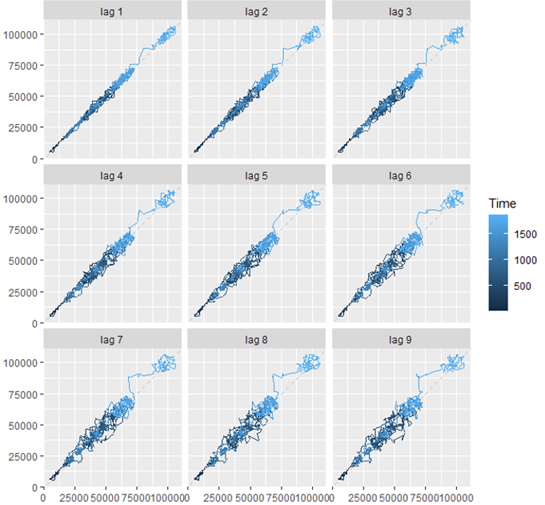
The time series of the Bitcoin-adjusted close price during and after the COVID-19 pandemic outbreak from January 1, 2020, to February 3, 2025, was modeled using the ARIMA model and R statistical software for Windows (version: 4.4.2). Figure 3 shows a scatterplot that plots the data points of this model along with the lags 1 to 9. All nine lag plots indicate that the data points are not random and have a linear trend. Moreover, no outliers appear in the dataset as all the data points lie close to each other, along a trend line. Since there is a clear and strong linear pattern along which the data points are plotted, an autocorrelation exists in the data; therefore, an auto-regressive model is suitable to model this time series. This shows that the ARIMA model used in this study is suitable.

Figure 3

Figure 3 The Lag Plot of Bitcoin-Adjusted Close Price During and After the COVID-19 Pandemic Outbreak

 

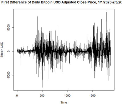
The augmented Dickey-Fuller (DF) test statistic of the Bitcoin time series model during and after the COVID-19 pandemic (January 1, 2020 -February 3, 2025) is -1.073 for this model. The p-value of 0.927 at a lag order of 12 indicates that the model fails to reject the null hypothesis of the DF test (H0: The time series is non-stationary). Therefore, the time series is non-stationary. The time series is converted to stationary by first-order difference (d = 1). As shown in Figure 4, the first difference obtained as a result has no trend, and overall, the plot remains symmetric around zero along the y-axis. This indicates that the time series obtained after the first-order difference is stationary.

 Figure 4

Figure 4 First-order Difference in the Bitcoin-Adjusted Close Price During and After the COVID-19 Pandemic Outbreak

 

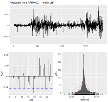
The fitted model is calculated auto. Arima() function in R and as a result, ARIMA (0,1,1) with drift model is fitted. The Ljung-Box Q-test statistic = 21.856 with df = 9 of this models has a p-value of 0.009347, which is less than 0.05, concluding that the residuals generated by the model are random and the ARIMA(0,1,1) with drift model fits the data well. The residuals, PACF, and residuals histogram are presented in Figure 5. The first graph at the top shows that the residuals are random and have no trend as they spread symmetrically along the horizontal line at the value = 0. The Error histogram shows that the residuals are normal and not skewed. They are also evenly distributed on either side of the bell curve.

Figure 5

 

Figure 5 The Residuals, PACF, and Residuals Histogram of ARIMA(0,1,1) with Drift During and After the COVID-19 Pandemic

The auto. Arima() function selects the model with the lowest AIC. In this case, ARIMA(0,1,1) with drift model has the lowest AIC and is then chosen to fit the time series. The RMSE of the model is 1342.093 (MSE is 1,801,213.62) with BIC = 32093.42 and AIC = 32076.84. In this case, ARIMA(0,1,1) with drift is a simple exponential smoothing with growth model. The ARIMA(0,1,1) model with constant has the following prediction equation:

 

 

The one-period-ahead forecasts from this model are qualitatively like those of the SES model, except that the long-term forecast trajectory is typically a sloping line rather than a horizontal line. Figure 6 shows the predicted and observed values of the time series.

Figure 6

Figure 6 Observed and Predicted Bitcoin-Adjusted Close Price During and After the COVID-19 Pandemic Using ARIMA(0,1,1) with Drift

 

4.2. ARIMA-NARNN HYBRID MODEL

The residuals obtained from the ARIMA model generated using R statistical software for Windows (version: 4.4.2) were subjected to hybrid modeling using MATLAB for Windows (version: 2024a). The residuals of the ARIMA model used to fit the time series data from January 1, 2020, to February 3, 2025, were used in NARNN modeling. In this study, the statistical analysis software MATLAB for Windows (version: R2024a) was used to model the Bitcoin time series using the LM training algorithm.

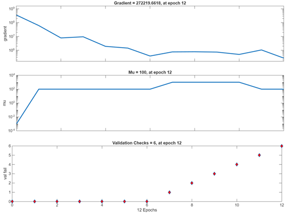
In the hybrid model, the linear component of the Bitcoin-adjusted close price time series is modeled using ARIMA in R programming software. The residuals that result from the ARIMA models fitted earlier in the study contain the time series’ nonlinear component. These residuals are passed through the NARNN model to reduce the errors by minimizing the mean squared error (MSE), given their promising performance in modeling nonlinear time series data using MATLAB programming software. The number of hidden neurons and the delays are chosen by experiments, and the LM training algorithm is used to train the model Table 1, Table 2, Figure 7 and Figure 8).

Table 1

Table 1 Time Series Training Process of the Hybrid Model
Unit	Initial Value	Stopped Value	Target Value
Epoch	0	12	1000
Elapsed Time	-	00:00:01	-
Performance	8.83E+07	1.77E+06	0
Gradient	3.57E+08	2.72E+05	1.00E-07
Mu	0.001	100	1.00E+10
Validation Checks	0	6	6

 

Table 2

Table 2 Time Series Validation Performance of the Hybrid Model
	Observations	MSE	R
Training	1301	1.78E+06	0.1557
Validation	279	1.77E+06	0.0331
Test	279	1.77E+06	0.0651
Training data: 70% Validation data: 15% Test data: 15%
Training algorithm: Levenberg-Marquardt
Training Results (Layer size: 10, Time delay: 2)
Performance: Mean squared error

 

Figure 7

Figure 7 Time Series Training Process of the Hybrid Model During and After the COVID-19 Pandemic Outbreak

 

Figure 8

 

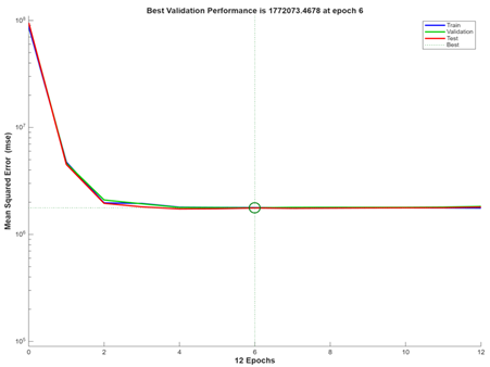
Figure 8 Time Series Validation Performance of the Hybrid Model During and After the COVID-19 Pandemic Outbreak

 

The residuals generated by the ARIMA(0,1,1) with drift model developed earlier in this study to fit the linear component of the Bitcoin-adjusted close price time series during and after the COVID-19 pandemic (January 1, 2020 – February 10, 2024) are passed through the NARNN model as these residuals form the nonlinear component of the Bitcoin time series. The hybrid model trained using the LM algorithm yielded the least MSE of 1.7814e+06 at the number of hidden neurons = 10 and the number of time delays = 2. Specifically, 10 Neurons in the Hidden Layer means that the NARNN part of the model has 10 processing units in its hidden layer, allowing it to learn complex nonlinear relationships, and 2 Time Delays means that the NARNN model uses the past two observations to predict the next value, helping it capture short-term dependencies in the data.

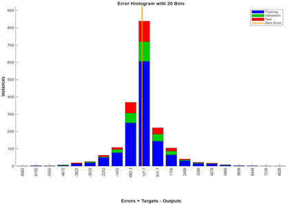
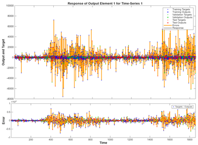
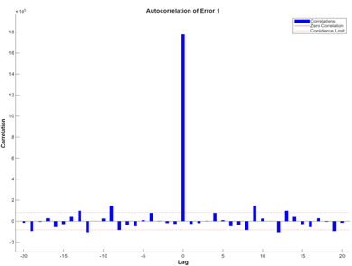
Figure 9 shows the time-series response of this hybrid model. The model predicts the data well in training, validation, and test sets. The errors are also close to the zero marks, which are evenly spread on either side. This indicates that the model has small errors. Figure 10 shows the time series plot of this hybrid model. The predicted (output) and observed (target) values are close for the majority of the observations and are distributed across both sides. The errors form along a horizontal line at 0 and are located close to the zero marks, indicating that the errors are small. The error autocorrelation in Figure 11 shows a spike at lag = 0 and is approximately within the 95% confidence interval for other lag numbers. At some lag numbers, the correlation goes beyond the confidence intervals, indicating that the model could be improved.

 Figure 9

Figure 9 Time Series Error Histogram of the Hybrid Model During and After the COVID-19 Pandemic

 

Figure 10

Figure 10 Time-Series Response of the Hybrid Model During and After the COVID-19 Pandemic

 

Figure 11

 

Figure 11 Error Autocorrelation of the Hybrid Model During and After the COVID-19 Pandemic

 

5. DISCUSSION

A range of factors, including market sentiment, macroeconomic trends, regulatory developments, and technological advancements, influenced the price volatility of Bitcoin. Unlike traditional financial assets, Bitcoin lacks intrinsic value and is largely influenced by speculative trading, making price movements highly unpredictable. This high level of volatility poses significant challenges for investors and financial institutions, as sudden price swings can lead to substantial gains or losses within short timeframes. Consequently, effective risk management in Bitcoin investments requires sophisticated forecasting techniques that can capture both the predictable and unpredictable components of price fluctuations.

Risk management in Bitcoin trading involves identifying, analyzing, and mitigating financial risks to minimize potential losses. Traditional risk management strategies, such as portfolio diversification, stop-loss mechanisms, and hedging, provide a foundational approach. However, given the extreme price fluctuations of Bitcoin, advanced data-driven techniques are increasingly necessary to complement these conventional strategies. Accurate predictive modeling allows investors to make informed decisions, optimize entry and exit points, and mitigate exposure to downside risks. In this regard, ML and statistical models play a critical role in enhancing risk assessment.

The ARIMA-NARNN hybrid model is a powerful tool for forecasting Bitcoin prices, as it leverages the strengths of both linear and nonlinear modeling techniques. ARIMA is well-suited for capturing linear trends and temporal dependencies within time series data, while NARNN excels at detecting complex, nonlinear patterns that may be overlooked by traditional statistical models. By combining these two methodologies, the hybrid approach compensates for the limitations of each individual model, producing more accurate and reliable price forecasts. This enhanced predictive capability is particularly valuable in volatile markets, such as Bitcoin, where price movements are influenced by a combination of historical trends and unpredictable external factors.

Moreover, the integration of ARIMA and NARNN improves the robustness of forecasting models, enabling traders and institutional investors to develop more effective risk mitigation strategies. With more precise predictions, investors can implement dynamic trading strategies that adapt to market conditions, reducing exposure to unexpected downturns. Furthermore, businesses that accept Bitcoin as a payment method can use such forecasting techniques to minimize financial uncertainty, ensuring better pricing and risk assessment mechanisms. The ability to anticipate price fluctuations enhances financial stability in the cryptocurrency ecosystem for both individual and institutional participants.

Ultimately, the Hybrid model’s predictive accuracy plays a crucial role in shaping strategic financial decisions in the Bitcoin market. As the adoption of cryptocurrency continues to grow, the development and refinement of advanced forecasting techniques will become increasingly essential for managing financial risk. By leveraging hybrid models that integrate linear and nonlinear analyses, investors and businesses can confidently navigate Bitcoin’s inherent volatility, making data-driven decisions that enhance financial resilience.

 

6. CONCLUSION

The COVID-19 pandemic outbreak had a massive impact on the economy and financial ecosystem of the United States and the world. A global shuffle in the financial markets and the economic balance has caused a dramatic change to the already volatile Bitcoin value in USD. Due to this dramatic and drastic change in the trend of the Bitcoin-adjusted close prices during and after the COVID-19 pandemic outbreak, traditional forecasting models, such as ARIMA, may not be as efficient or accurate as they used to be. Conversely, the ARIMA-NARNN hybrid model finds more relevance in forecasting future Bitcoin prices as it performs better than the more commonly used forecasting model, i.e., ARIMA.

This study aimed to identify the most suitable model for analyzing the time series data of daily Bitcoin-adjusted close price during and after the COVID-19 pandemic (January 1, 2020 - February 3, 2025). In this study, the suitable time series model was determined to be the ARIMA-NARNN hybrid model, as it exhibited the lowest AIC values among the various models considered. Notably, this ARIMA-NARNN hybrid model provided compelling evidence that the future daily Bitcoin-adjusted close price will increase over time.

Empirically, the ARIMA and NARNN models have demonstrated proficiency in modeling linear and nonlinear time series data, respectively. However, opting for a hybrid model, which combines the strengths of ARIMA and NARNN, offers a compelling advantage. This hybrid approach seamlessly integrates linear and nonlinear modeling capabilities, making it a superior choice for accurately modeling complex time series data.

The comparative analysis revealed that the hybrid model, featuring 10 neurons in the hidden layer and 2-time delays, outperformed the ARIMA(0,1,1) with drift model (MSE = 1.8012e+06). The hybrid model achieved the highest accuracy with an MSE of 1.7814e+06, indicating its superior predictive capability for daily Bitcoin-adjusted close price. According to the findings of this study, the hybrid model not only enriches the available information but also holds significant importance for decision-making processes concerning the future forecast of Bitcoin. Furthermore, different forecast combinations of time series models, such as neural networks, could be used to check their efficiency in forecasting Bitcoin prices and other volatile time series. More research in this direction could help discover more efficient forecasting models.

 

CONFLICT OF INTERESTS

None. 

 

ACKNOWLEDGMENTS

None.

 

REFERENCES

Atsalakis, G. S., Atsalaki, I. G., Pasiouras, F., & Zopounidis, C. (2019). Bitcoin Price Forecasting with Neuro-Fuzzy Techniques. European Journal of Operational Research, 276(2), 770–780. https://doi.org/10.1016/j.ejor.2019.01.040

Ayaz, Z., Fiajdhi, J., Sabah, A., & Ansari, M. (2020). Bitcoin Price Prediction Using ARIMA Model. TechRxiv, 1–10. https://doi.org/10.36227/techrxiv.12098067.v1

Boozary, P., Sheykhan, S., & GhorbanTanhaei, H. (2025). Forecasting the Bitcoin Price Using the Various Machine Learning: A Systematic Review in Data-Driven Marketing. Systems and Soft Computing, 7, Article 200209, 1–13. https://doi.org/10.1016/j.sasc.2025.200209

Denton, J. W. (1995). How Good are Neural Networks for Causal Forecasting. The Journal of Business Forecasting Methods & Systems, 14, 17.

Dowe, D. L., Peiris, S., & Kima, E. (2025). A Novel ARFIMA-ANN Hybrid Model for Forecasting Time Series—and its Role in Explainable AI. Journal of Econometrics and Statistics, 5(1), 107–127.

Fathi, O. (2025). Time Series Forecasting Using a Hybrid ARIMA and LSTM Model. Velvet Consulting.

Hajirahimi, Z., & Khashei, M. (2023). Hybridization of Hybrid Structures for Time Series Forecasting: A Review. Artificial Intelligence Review, 56, 1201–1261. https://doi.org/10.1007/s10462-022-10199-0

Hao, Y., & Gao, Q. (2020). Predicting the Trend of Stock Market Index Using the Hybrid Neural Network Based on Multiple Time Scale Feature Learning. Applied Sciences, 10(11), 3961. https://doi.org/10.3390/app10113961

Hozjan, V. (2025, February 25). Bitcoin: From birth to Global Recognition. NiceHash.

Laurent, D. (2025, February 25). The History of Bitcoin: From Inception to Mainstream Adoption. WoolyBlog.

Levenberg, K. (1944). A Method for the Solution of Certain Non-Linear Problems in Least Squares. Quarterly of Applied Mathematics, 2(2), 164–168. https://doi.org/10.1090/qam/10666

Luc Minh, T., Senkerik, R., & Dang, T. K. (2024). Predicting Bitcoin's Price: A Critical Review of Forecasting Models and Methods. In T. K. Dang, J. Küng, & T. M. Chung (Eds.), Future Data and Security Engineering. Big Data, Security and Privacy, Smart City and Industry 4.0 Applications FDSE 2024 (Vol. 2309). Springer. https://doi.org/10.1007/978-981-96-0434-0_3

Marquardt, D. W. (1963). An Algorithm for Least-Squares Estimation of Nonlinear Parameters. Journal of the Society for Industrial and Applied Mathematics, 11(2), 431–441. https://doi.org/10.1137/0111030

Ponciano, J. (2025, February 25). Tesla's Bitcoin Investment fell $1 billion last quarter amid crypto market crash. Forbes.

Portfolio Insider. (2025, February 25). Can Bitcoin Grow Faster than the Internet? Nasdaq.

Prajapati, S., Swaraj, A., Lalwani, R., Narwal, A. A., & Verma, K. (2021). Comparison of Traditional and Hybrid Time Series Models for Forecasting COVID-19 cases. arXiv, 1–14. https://doi.org/10.21203/rs.3.rs-493195/v1

Russolillo, S. (2025, February 25). Bitcoin Goes to the Big Four: PWC Accepts First Digital-Currency Payment. The Wall Street Journal.

Yenidogan, I., Cayır, A., Kozan, O., Dag, T., & Arslan, C. (2018). Bitcoin Forecasting Using ARIMA and PROPHET. In Proceedings of the 3rd International Conference on Computer Science and Engineering (UBMK), Bosnia. https://doi.org/10.1109/UBMK.2018.8566476

Yu, L., Zhou, L., Tan, L., Jiang, H., Wang, Y., Wei, S., & Nie, S. (2014). Application of a New Hybrid Model with Seasonal Auto-Regressive Integrated Moving Average (ARIMA) and Nonlinear Auto-Regressive Neural Network (NARNN) in Forecasting Incidence Cases of HFMD in Shenzhen, China. PLOS One, 9(6), e98241. https://doi.org/10.1371/journal.pone.0098241

Zhang, G. P. (2003). Time Series Forecasting Using a Hybrid ARIMA and Neural Network Model. Neurocomputing, 50, 159–175. https://doi.org/10.1016/S0925-2312(01)00702-0